Linear Algebra for Machine Learning using Python

Linear algebra is one of the most beautiful subjects one will come across if understood. I learned it from lectures by Prof Gilbert Strang from MIT who has an enthusiastic and thought-provoking way of explaining the subject.

If you want to get a deeper understanding of the subject I would recommend you check out Gilbert Strang’s online lectures.

I would highly recommend to check out Linear Algebra Playlist by 3Blue1Brown for a visual understanding feast.

According to Wikipedia :

“ Linear Algebra is the branch of mathematics concerning linear equations and their representations in vector spaces and through matrices ”

This article is a comprehensive review of the subject tailored to data science learners.

You may choose to skip the parts you are already familiar with.

Why should Data Scientists learn Linear Algebra?

In terms of mathematical prerequisites, linear algebra ranks on the top because it’s a building block for a lot of algorithms and is like a language to write equations about high dimensional data.

Linear algebra is also used in most sciences and fields of engineering, because it allows modeling many natural phenomena, and computing efficiently with such models.

Data scientists deal with data either to analyze it to get insights or to visualize and learn from it. An efficient way to represent that enormous amount of data using simple mathematical equations is through linear algebra.

You can turn a system of thousand linear equations having a thousand variables to a simple Ax=b equation and then use standard algorithms to solve the same. 

The reasons for studying linear algebra :

1. Linear algebra provides a system for multivariate representation of data as vectors and tensors
2. The vector and tensor representation is a core part of many machine learning algorithms like Principal Component Analysis, Neural Networks, etc. 
3. Being familiar with the linear algebra language helps in reading research papers as well as their implementation in the space of AI and Data Science

Where it’s commonly used?

1. Neural Network → Matrix Operations
2. Dimensionality Reduction using PCA and Powers of Matrices → Eigenvalues
3. Multivariate Calculus and Probability → higher-order representation
4. Second-order Hessian Based optimization methods → Solving Ax=b

If you are not familiar with these, don’t worry and keep going. 

What to learn?

Building Blocks

It's just like basic algebra where you have variables and constants as your building blocks where we used to convert a real-world problem into an algebraic one. In linear algebra, the building blocks are vectors and tensors which can be used to represent data or a system of linear equations in order to solve a real-world problem.

Vectors

A Vector is the most fundamental building block of linear algebra. A collection of items can be thought of as a vector that also has a geometrical meaning associated with it. Vectors can be thought to be existing in n-dimensional space (n being the number of elements in that vector). A vector is always a column rather than a row in linear algebra conventions.

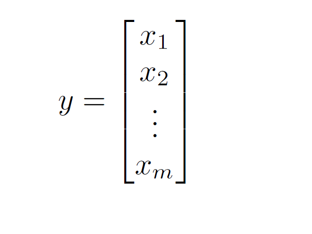
Like we studied about vectors in physics, they have magnitude and a direction that depends upon those collection of numbers and their relative proportioning.

For people who code → Vectors are just one-dimensional arrays with a geometrical meaning

In python, we use the NumPy library for linear algebra. 

import numpy as np
vector = np.random.rand(3)
vector
array([0.2459582 , 0.98466978, 0.63681196])

Here we generate a random vector, you can also generate the by putting number manually like :

a=np.array([1,3,4])

Tensors

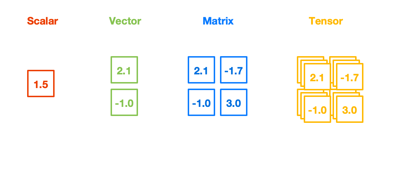
Tensors are a general extension to vectors. You may call a vector as a one-dimensional tensor, to begin with.

Tensors can be thought of as a collection of vectors. You can arrange vectors in a row to get a two-dimensional tensor commonly known as a matrix. Every column is a vector in that matrix, that’s the way you gotta think every time (column picture).

import numpy as np

# Creating two random 3X3 matrices
A=np.random.randint(10,size=(3,3))
B=np.random.randint(10,size=(3,3))

A
array([[7, 5, 3],
       [9, 9, 6],
       [6, 8, 4]])
B
array([[5, 5, 0],
       [0, 3, 2],
       [1, 6, 2]])

The collection of matrices (2D Tensor) can be thought of as 3D tensor, and the concept can be extended to N-Dimensional tensors. Google’s TensorFlow framework was actually named after tensors and is the building block for representing high dimensional and its operations. 

For people who code → Tensors are just n-dimensional arrays with a mathematical  meaning

Let’s initialize a 3-dimensional tensor using the NumPy library in python of size  [2, 3, 4] which can be thought as 2 matrices of size [3, 4]

np.random.randint(10,size=(2,3,4))

array([[[7, 0, 5, 0],
        [6, 6, 8, 6],
        [6, 8, 6, 2]],

       [[7, 8, 3, 6],
        [0, 8, 4, 9],
        [6, 7, 6, 4]]])

Matrix Operations

We are going to discuss matrix operations briefly, but there is something called as tensor algebra as well for n-dimensional tensors. The most common operations include addition, subtraction, multiplication, transpose, and inverse.  

You can add and subtract matrices element-wise, no-frills. But for multiplication, you can have either element-wise multiplication or matrix multiplication. For element-wise multiplication, you can multiply each corresponding element just like addition or subtraction.

# Using A and B defined earlier
A
array([[7, 5, 3],
       [9, 9, 6],
       [6, 8, 4]])
B
array([[5, 5, 0],
       [0, 3, 2],
       [1, 6, 2]])

#Basic operations
A+B             	# Add
array([[12, 10,  3],
       [ 9, 12,  8],
       [ 7, 14,  6]])

A*B             	# Element Wise Multiplication
array([[35, 25,  0],
       [ 0, 27, 12],
       [ 6, 48,  8]])

A@B             	# Matrix Product
array([[ 38,  68,  16],
       [ 51, 108,  30],
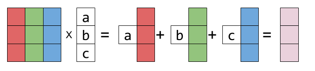
       [ 34,  78,  24]])

But In linear algebra matrix multiplication is referred to where you take a linear combination of vectors, which is an important concept in linear algebra.

If one vector is equal to the sum of scalar multiples of other vectors, it is said to be a linear combination of the other vectors.

$$C=AB $$

$$C_{ij}=\sum_{k}A_{ik}B_{kj}$$

Matrix multiplication is not commutative.

$$AB \neq BA$$

Transpose

The transpose is an important operation on a matrix which is just about taking its mirror image across the diagonal line (Line joining upper left corner to the lower right corner). So, basically the row values exchange with the column values.

$$A^T_{ij}=A_{ji}$$

A                    
array([[7, 5, 3],
       [9, 9, 6],
       [6, 8, 4]])

A.T                   # Transpose
array([[7, 9, 6],
       [5, 9, 8],
       [3, 6, 4]])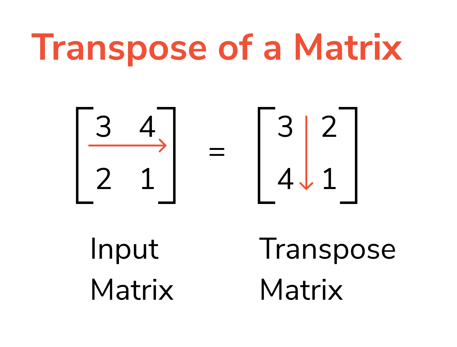

Matrix is called to be symmetric if its transpose is the same as itself. Another way is to say that both the lower triangular matrix and the upper triangular matrix are identical. If the blocks are negative of each other it’s called a skew-symmetric then.

Inverse

The inverse of a matrix is one which when multiplied with the original matrix results in an identity matrix (analogous to multiplying a variable with its reciprocal to get one as a result in normal algebra)

$$AA^{-1} = I$$

A
array([[7, 5, 3],
       [9, 9, 6],
       [6, 8, 4]])

np.linalg.inv(A)     			# Inverse
array([[ 0.4 , -0.13, -0.1 ],
       [ 0.  , -0.33,  0.5 ],
       [-0.6 ,  0.87, -0.6 ]])

The identity matrix contains the value one along the diagonal and zeros elsewhere.

$$AI=A$$

Identity = np.eye(3)

De Morgan’s Law

$$A^{-1}B^{-1}=(BA)^{-1}$$

You can verify this equation in python using the code mentioned below.

np.round(np.linalg.inv(A)@np.linalg.inv(B))==np.round(np.linalg.inv(B@A))

array([[ True,  True,  True],
       [ True,  True,  True],
       [ True,  True,  True]])

One of the analogies that stuck with me to remember this equation mentioned by Gilbert Strang during his lectures was that you wear socks first and then shoes, but when removing the duo, you remove the shoes first and then the socks.

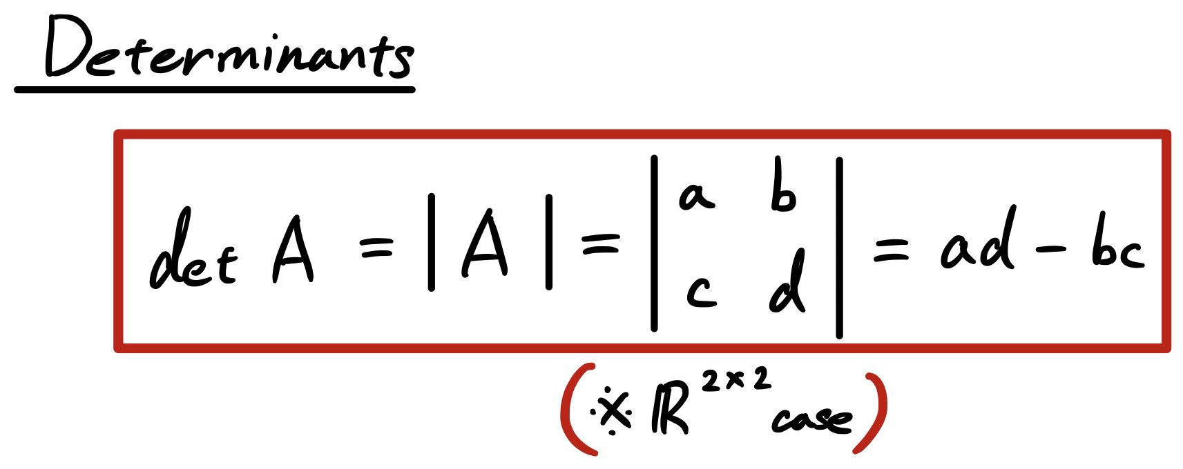
Determinant

the determinant is a scalar value that can be computed from the elements of a square matrix and encodes certain properties of the linear transformation described by the matrix.

The determinant of a matrix A is denoted det(A), det A, or |A|.

There are other concepts like vector space, column space, null space, rank, row echelon form, dimension, and basis which I won’t go into. You can refer the same here.

In python, you can again use the numpy library for determinants.

A
array([[7, 5, 3],
       [9, 9, 6],
       [6, 8, 4]])
       
np.linalg.det(A)    # Determinant
-30

System of Linear equations

The fundamental problem in linear algebra is to solve n linear equations with n unknowns.

We could use the method of elimination or substitution to solve for them manually for equations with two or three variables but using a matrix approach to do the same is a formal way of doing especially for using the computers to the hard work for solving them.

Algorithms for solving these equations efficiently are one of the most important tools in physics, engineering, and obviously data science. A lot of nonlinear problems can be converted to linear problems. Linear functions are the best to operate with and most functions are nonlinear but are locally linear.

$$Ax=b$$

A lot of research has gone into solving these set of equations efficiently through computers with respect to orders of complexity. There are both analytical as well as approximate (numerical) methods to solve the problem.

Inverse Method

You can simply solve \(Ax=b\) equations by calculating the inverse of A and multiplying it with b but the problem is that it’s not an efficient way to solve the problem because inverse computation is expensive for larger values of n which is basically the number of equations I.e. time complexity is bad.

An important thing to note is that the inverse should exist (nonsingular matrix) for a solution to the system of equations. Another way of saying the same is to say that the vectors (columns of the matrix) should be linearly independent.

If no vector in the set can be written as a linear combination of other vectors, then the vectors are said to be linearly independent.

A=np.random.randint(10,size=(3,3))
b=np.random.randint(10,size=(3,1))

A=np.random.randint(10,size=(3,3))
array([[5, 3, 0],
       [7, 1, 0],
       [1, 5, 1]])

b=np.random.randint(10,size=(3,1))
array([[0],
       [5],
       [5]])

import time
tic=time.time()
x=np.linalg.inv(A)@b      # Solving Ax=b using inverse
toc=time.time()
print(x)
print("Using Inverse: " + str((toc-tic)*1000) + "ms")

import time
tic=time.time()
x=np.linalg.inv(A)@b      # Solving Ax=b using inverse
toc=time.time()

print(x)
[[ 0.9375]
 [-1.5625]
 [11.875 ]]

print("Using Inverse: " + str((toc-tic)*1000) + "ms")

Using Inverse: 0.92ms

Gaussian Elimination

Gaussian elimination is one of the most popular methods to solve them with an order of complexity of \(n^3\). It is very similar to the elimination method used to solve the linear system of equations manually but instead is an algorithm way to solve the set of equations. I won’t go into details regarding solving the same but you can refer Gilbert Strang's Course to go into more detail.

tic=time.time()
x=np.linalg.solve(A,b)    # Solving Ax=b using built in solver 
toc=time.time()
print(x)
print("Gaussian Elimination: " + str((toc-tic)*1000) + "ms")

Gaussian Elimination: 0.5948543548583984ms

As you can see, gaussian elimination or other efficient algorithms are much better than solving using the inverse in terms of time. The difference becomes significant for larger matrices.

Eigenvalue Decomposition

The second most important and useful concept in linear algebra after solving the system of linear equations is that of eigenvalue decomposition.

Eigenvalue Applications in Machine Learning and data science would be for Principal Component Analysis (PCA), spectral clustering and many more.

Eigenvalues and eigenvectors are special numbers that define a matrix and are considered by some as the soul of it.

So, basically for a special vector x, its matrix product with the original matrix A gives the result as a scalar multiple of \(x\). So the matrix A transforms the special vector \(x\) (eigenvector) in such a way that it scales in the same direction by a factor known as an eigenvalue.

$$Ax=\lambda x$$

To solve this particular equation manually, the equation can be written simply as

$$(A-\lambda I) x=0$$

And for non zero value x and non zero null space, determinant of $A-\lambda I$ has to be zero.

$$|A-\lambda I|=0$$

Solving that equation gives an nth degree polynomial equation I.e. quadratic equation when the size of A is [2 X 2]. So, we’ll have n eigenvalues and n corresponding eigenvectors when the size of A is [n X n].

But there are computational methods for finding the pair of eigenvectors and eigenvalues.

A=np.random.randint(10,size=(3,3))
A_sym=(A+A.T)/2                    # Symmetric Matrix ~ real eigenvalues 
eigenvalues, eigenvectors = np.linalg.eig(A_sym)

A_sym
array([[0. , 1. , 6. ],
       [1. , 4. , 3.5],
       [6. , 3.5, 7. ]])

eigenvalues
array([12.01, -3.56,  2.55])

eigenvectors
array([[-0.44, -0.84,  0.32],
       [-0.41, -0.13, -0.9 ],
       [-0.8 ,  0.52,  0.29]])

There are some results with respect to eigenvalues which can be really helpful

$$Trace(A) = \sum_{i}A_{ii} = \sum_{i}\lambda_i$$

np.sum(np.diag(A_sym))
11.0

np.sum(eigenvalues)
11.0

Trace [A] = sum of diagonal entries of A = sum of all eigenvalues

The determinant of A is just the product of all the eigenvalues.

$$det(A)=\prod_{i}\lambda_i$$

np.prod(eigenvalues)
-109.00

np.linalg.det(A_sym)
-108.99

Isn’t that just wonderful to have? These two equations can help you to do a fast sanity check. For just two eigenvalues, these two equations are enough to get that quadratic equation.

EigenValue Decomposition

Like any decomposition, eigenvalue decomposition breaks the matrix as a product of matrices. It’s also known as diagonalization of A and is very useful for a lot of applications

So, it looks similar to the equation \(Ax=\lambda x\) we discussed above, the only difference being instead of vector x we take all the eigenvectors (n) as columns to put in a matrix S. And the V being the diagonal matrix containing the eigenvalues in the diagonals.

$$AS=S\Lambda$$

np.round(A_sym@eigenvectors)==np.round(eigenvectors@(eigenvalues*np.eye(3)))

array([[ True,  True,  True],
       [ True,  True,  True],
       [ True,  True,  True]])

$$A=S\Lambda^{-1}S$$

Using python, we were able to do this decomposition in just a single line of code where we input the matrix A to get EigenVectors( \(S\) ) and EigenValues( \(\Lambda\) ) as outputs.

Powers of A

One really important benefit of decomposing the matrix into eigenvectors and eigenvalues is in calculating the powers of A efficiently. If I want to calculate \(A²\), I can just have a matrix product but for higher powers of A like \(A^{100}\) it’s much more computationally efficient to perform eigenvalue decomposition and then take just powers of eigenvalues since the Eigenvectors remain the same (so helpful).

So, basically the equation looks like

$$A^{n}=S\Lambda^{n}S^{-1}$$

Let’s take an example of calculating \(A³\) using matrix multiplication and Eigenvalue decomposition.

import time
tic=time.time()
A_cube=A_sym@A_sym@A_sym            # Calculating by matrix multiplication
toc=time.time()
print(A_cube)
print("Using Matrix Multiplication: " + str((tic-toc)*1000 +"ms")

tic=time.time()
A_cube=eigenvectors@((eigenvalues**3)*np.eye(3))@np.linalg.inv(eigenvectors) # Calculating by eigenvalue decomposition
toc=time.time()
print(A_cube)
print("Using EigenValue Decomposition: " + str((tic-toc)*1000 +"ms")

Let me share some other important results regarding our discussion.

If A is symmetric then eigenvalues are real and eigenvector matrix is actually orthonormal

Eigenvalues for the transposed matrix is the same

Eigenvector matrix for powers of the matrix A remains the same

$$\lambda_{A^{-1}} = \frac{1}{\lambda_A}$$

Two vectors in an inner product space are orthonormal if they are orthogonal, or perpendicular along a line, and unit vectors. A set of vectors form an orthonormal set if all vectors in the set are mutually orthogonal and all of unit length.

$$AA^{T}=I$$

$$A^{-1}=A^{T}$$

Singular Value Decomposition and Pseudo Inverse

Eigenvalue decomposition and many others are for square matrices only. Along with that inverse of a matrix is defined for square matrices as well. But in actual practice, we deal with rectangular matrices as well.

So, instead of eigenvalue decomposition, singular value decomposition can be used for similar purposes and pseudo-inverse instead of our normal inverse.

[similarity with eigenvalue decomposition is important]

$$A=UDV^{T}$$

Here’s another application of eigenvalue decomposition, it helps in singular value decomposition.

$$U=Eigenvectors(AA^{T})$$

$$V=Eigenvectors(A^{T}A)$$

$$D=\sqrt{Eigenvalues(AA^{T})}$$

\(U\), \(D\) and \(V^T\) have shapes [m, m], [m, n], and [n, n] respectively where [m, n] is the shape for A.

A=np.random.randint(10,size=(2,3))
U,D,Vt = np.linalg.svd(A)

A
array([[7, 1, 3],
       [4, 6, 6]])

U
array([[-0.60473171, -0.79642926],
       [-0.79642926,  0.60473171]])

D
array([11.29087215,  4.41771504])

Vt
array([[-0.65706518, -0.47678401, -0.58390269],
       [-0.71441412,  0.64104655,  0.28048492]])

U@np.diag(D)@Vt
array([[7., 1., 3.],
       [4., 6., 6.]])

The good thing about singular value decomposition is that they can used for matrix inversion for rectangular matrices which brings us to the concept of a Pseudo-Inverse.

Pseudo Inverse

It’s the inverse equivalent for rectangular matrices. So, as know using Singular Value Decomposition we get

$$A=UDV^{T}$$

Using SVD we get the pseudo inverse as

$$A^{+}=VD^{+}U^{T}$$

You can use the linear algebra library in python to get it directly by just using pinv rather than the inv.

A=np.random.randint(10,size=(2,3))
A_pinv=np.linalg.pinv(A)

$$AA^{+}=I$$

A
array([[5, 5, 3],
       [7, 0, 4]])

A_pinv
array([[-0.00246002,  0.10947109],
       [ 0.199877  , -0.14452645],
       [ 0.00430504,  0.05842558]])

np.round(A@A_pinv,2)
array([[ 1.,  0.],
       [-0.,  1.]])

Norm

Norms are to measure the size of a vector, similar to what magnitude is. But the magnitude of a vector we know from physics classes is just a subset of the same.

We have \(L_1\) norm, \(L_2\) norm, and so on.. We can generalize it as \(L_p\) norm which is defined as for vectors

$$\|x_p\|=(\sum_{i}|{x_i}|^p)^{\frac{1}{p}}$$

x=np.random.rand(3)
x_l2 = np.linalg.norm(x)
x_l1 = np.linalg.norm(x,1)

x
array([0.57427356, 0.71951852, 0.71032612])

x_l1
2.004

x_l2
1.162

And we also have infinity norm as p tends to infinity, defined as

$$\|x\|_{\inf}=max|x_i|$$

For matrices, we can have a similar metric known as the Frobenius norm which is defined as

$$\|A\|_{F}^2=\sum_{i}\sum_{j}A_{ij}^2$$

A=np.random.randint(10,size=(2,2))
A_Frobenius=np.linalg.norm(A)

A
array([[6, 7],
       [1, 2]])

A_Frobenius
9.486

An alternate way of calculating Frobenius norm is through trace

$$\|A\|_F=\sqrt{Tr(AA^{T})}$$

Resources to refer

1. Deep Learning book  by  Ian Goodfellow
2. Linear Algebra and its Applications by Gilbert Strang
3. Linear Algebra Course  by Gilbert Strang MIT OCW
4. 3Blue 1Brown Youtube Channel
5. numpy.linalg Library

You can follow me on LinkedIn and Twitter.

I write articles related to personal development, AI & Data Science, and whatever I think is worth sharing :)